A Beginner-Friendly Introduction to Monte Carlo Method
Analyzing the Bitcoin Trend with Monte Carlo Simulations


Ok guys, we will be having a look at how to use the Monte Carlo Method to simulate financial trends. First we will be starting out with a clean definition so that everyone is one the same page and then we will be moving into a practical interpretation.
A Monte Carlo simulation is a statistical method used to analyze the behavior and performance of a system or process. The underlying idea is to generate random inputs which will be fed into a respective system or process. The inputs are drawn from the probability distribution of the individual input features.
With the set of generated inputs, the likelihood of different outcomes is estimated. This is done by running the simulation multiple times and analyzing the results of each run to determine the most likely outcomes or events.
History
The Monte Carlo method has an interesting historical background. It was developed in the 1940s, the midst of World War II by Stanislaw Ulam and John von Neumann, two mathematicians who were working on the Manhattan Project to develop the first nuclear weapons.
Ulam and Neumann were looking for a way to simulate the behavior of complex systems, such as the impact of radiation on different materials, and came up with the idea of using random sampling to make predictions about the behavior of these systems.

The name "Monte Carlo" was inspired by the famous Monte Carlo Casino in Monaco, which was known for its use of randomness and probability in games of chance.
The term "Monte Carlo" was coined to describe the method because it involved using random sampling and statistical analysis to make predictions about the behavior of complex systems, much like how the casino used these principles to determine the odds of different outcomes in games of chance.
Nowadays Monte Carlo simulations are being used in a variety of industries and applications, including risk analysis, financial modeling, and optimization of complex systems.
Core concept of the Monte Carlo method
The core concept behind a Monte Carlo Simulation are multiple random sampling runs from a given set of probability distributions. These can be of any type, for example: Binomial, Chi-square. Student's t, Normal, and so on.
When performing a Monte Carlo simulation the typical pattern includes the following steps:
- Define how input components interact with each other and form an output.
- Determine the probability distribution for each input or variable, which represents the range of possible values and their likelihood of occurring.
- Generate a large number of random samples from the probability distribution of each input or variable.
- Simulate the the interactions of the input variables using the generated samples from the previous step.
- Analyze the results of the simulation to make predictions about the performance or behavior of the system or process. This may include calculating statistical measures such as mean, standard deviation, and confidence intervals.
- Repeat the simulation multiple times to increase the accuracy of the predictions and to account for the inherent variability and uncertainty in the data.
Example 1: Dice rolls - Simple Python Implementation

In order to give you guys an initial feeling of how to implement a Monte Carlo simulation we are starting out with a simple example. First we will be simulating a single dice and try to find out how likely it is for each dice face to show up.
Of course it is trivial, because we know that each side of a dice should have the same probability of facing the top, if the dice has not been tinkered with. However, it is a good example to get an idea of how the Monte Carlo method works.
Objective
Use Monte Carlo simulations to find out the probability of each dice face showing up when rolling a standard dice.
The code below defines first the probability distribution for the dice roll.
# Each number has an equal probability of being rolled
probability_distribution = [1, 2, 3, 4, 5, 6]
Then it runs the simulation for a specified number of iterations, and stores the results in a list.
# Set the number of simulations to run
num_simulations = 20000

# Initialize a list to store the results of the simulations
results = []

# Run the simulation
for i in range(num_simulations):
  # Generate a random sample from the probability distribution
  result = random.choice(probability_distribution)
  # Add the result to the list
  results.append(result)
Finally, It then calculates the frequency of each outcome and prints the results. We can see that occurrence frequencies vary between 16.41% and 17.04%. If we would increase the number of simulations, eventually each number 1, 2, 3, 4, 5, 6 would have a probability 16.6666% of showing up.
# Calculate the frequency of each outcome
outcome_frequency = {}
for outcome in probability_distribution:
  outcome_frequency[outcome] = results.count(outcome)/num_simulations

print("Simulation results:")
for outcome, freq in outcome_frequency.items():
print(f"{outcome}: Occurrence {freq * 100:.2f}% ") 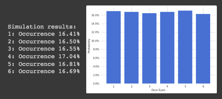
Bringing it all together, the full code looks as follows. Feel free to copy the code and try it out yourself.
Example 2: Bitcoin price forecasts - Advanced Python Implementation

After the initial example, we are now looking into a way more complex task. We are trying to predict future Bitcoin prices by simulating their future behaviour. At the end we will run multiple simulations to get an idea of how the Bitcoin price could potential change.
Objective
Use Monte Carlo simulations to find out how the Bitcoin prices can evolve in the future.
Load Bitcoin Prices
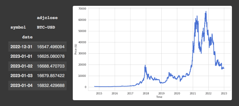
First, we are loading loading all historical Bitcoin prices on a daily increment level and drop all column except the Adjusted Closing Price of each day.
ticker = ['BTC-USD']

ticker_data = yq.Ticker(ticker, asynchronous=True)
prices = ticker_data.history(period='max', interval='1d',)
prices = prices.drop(['volume',	'high',	'open',	'low',	'close'], axis=1)
prices = prices.unstack(level=0).sort_index().fillna(method='ffill').bfill()
Printing the dataframe and plotting the price data over time the following two illustration show up.
Bitcoin Prices
Calculate Bitcoin Returns
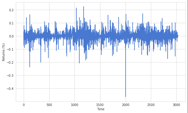
Since Bitcoin prices are not stationary at all, we have to convert the price data into price returns. This can be done by calculating the percentage change from one day to the next. In addition, all NaN values are dropped to prevent error messages down the road.
returns = np.log(1 + prices.pct_change())
returns.dropna(inplace=True)
returns = np.squeeze(returns.values)
Bitcoin Price Returns
Probability Distribution of Bitcoin Returns
Now that we have the price return data we can derive the probability distribution of the Bitcoin returns.
This step is crucial, since in most implementations financial asset returns are modelled with an assumed normal distribution. As you can see, the illustration below shows that Bitcoin returns are not normal distributed. Instead, the probability distribution has significantly heavier tails then a normal distribution. Not considering the higher probabilities for extreme daily returns (heavy tails) will lead to underestimation of significant losses. Thus, it is important to model the real distribution of a variable and not assume it is normal distributed.
distribution_kernel = kde.gaussian_kde(returns, bw_method='scott')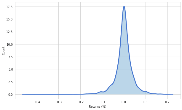
Monte Carlo Simulations for Bitcoin Price Forecasts
After having Bitcoin price returns and it's probability distribution in place we can start putting together the simulations.
In total we are running 100 simulations for the forecasting of Bitcoin returns and within each simulation we will predict 255 days (1 year of trading days) in the future. Thus, for each simulation we have to sample 255 returns form the return distribution.
Then the last actual Bitcoin price return which we calculated earlier is multiplied with an array of all sampled returns per simulation.
#Settings for Monte Carlo asset data, how long, and how many forecasts
t_intervals = 255 # time steps forecasted into future
iterations = 100 # amount of simulations
#Generate return samples in an array with the shape (t_intervals, iterations)
daily_sample_returns = np.empty((0,t_intervals))
for i in range(iterations):
daily_sample_returns = np.append(daily_sample_returns, distribution_kernel.resample(t_intervals)+1, axis=0)
daily_sample_returns = daily_sample_returns.T
#Takes last data point as startpoint point for simulation
price_list = np.zeros_like(daily_sample_returns)
price_list[0] = returns[-1]
#Apply Monte Carlo simulations
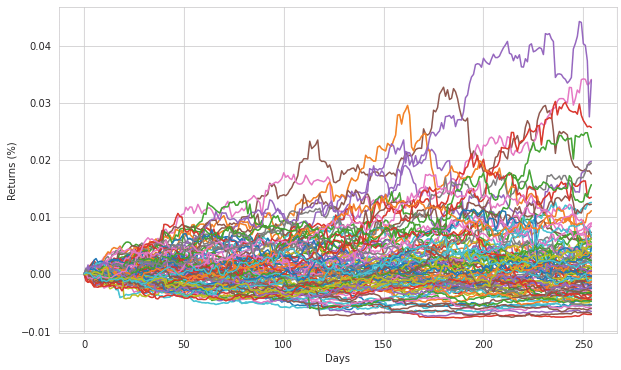
for t in range(1, t_intervals):
price_list[t] = price_list[t - 1] * daily_sample_returns[t]Repeating this for a 100 simulation and plotting it all out, we will receive the following chart. We can see that after 255 days the Bitcoin price could change with a return between roughly -0.05% and 3.5%.
Anyone, who wants to run the code him or herself, the link below redirects you to a Colab Notebook that you can copy and run end-to-end.
https://colab.research.google.com/drive/1IV9ay441983OJ8DcuSZ486y7yN3NzQw5?usp=sharing
I hope that these example are helping you guys to obtain an initial understanding of how to make use of a Monte Carlo simulation.
Application fields
The Monte Carlo method can be used in many other areas. The method in general useful for simulating systems that are characterized by a significant uncertainty in inputs and with many degrees of freedom. Areas of application include:
Finance
The Monte Carlo method is widely used in the finance field for a variety of purposes, including:
- Risk analysis: Monte Carlo simulations can be used to analyze the risk of different financial instruments, such as stocks, bonds, and derivatives. This can help investors and financial institutions understand the potential risks and rewards of different investments and make informed decisions about resource allocation.
- Portfolio optimization: Monte Carlo simulations can be used to evaluate the performance of investment portfolios and identify the optimal mix of assets to maximize returns while minimizing risk.
- Financial modeling: Monte Carlo simulations can be used to build complex financial models that take into account a wide range of variables and uncertainties, such as market movements, inflation, and interest rates. These models can be used to make predictions about the future performance of financial instruments and inform investment decisions.
- Option pricing: Monte Carlo simulations can be used to evaluate the value of financial options, such as call and put options, by simulating the underlying assets and analyzing the likelihood of different outcomes.
- Stress testing: Monte Carlo simulations can be used to test the robustness of financial models and identify potential risks and vulnerabilities under different market conditions. This can help financial institutions prepare for potential market shocks and reduce the likelihood of losses.
Engineering
The Monte Carlo method is widely used in the engineering field for a variety of purposes, including:
- Performance analysis: Monte Carlo simulations can be used to analyze the performance of aircraft, power plants, and manufacturing processes. This can help engineers understand the behavior of these systems under different conditions and identify potential problems or improvements.
- Reliability analysis: Monte Carlo simulations can be used to evaluate the reliability of mechanical systems, such as the likelihood of failure or maintenance needs, and identify potential problems or vulnerabilities.
- Safety analysis: Monte Carlo simulations can be used to analyze the safety of complex systems, such as the risk of accidents or malfunctions, and identify ways to reduce these risks.
- Environmental impact assessment: Monte Carlo simulations can be used to evaluate the environmental impact which is caused by emissions of greenhouse gases, and identify ways to reduce these impacts.
Physical Sciences
The Monte Carlo method is widely used in the physical sciences field for a variety of purposes, including:
- Molecular simulations: Monte Carlo simulations can be used to analyze the behavior of molecules, such as their movements and interactions, and predict the properties of different materials.
- Astronomy: Monte Carlo simulations can be used to analyze the behavior of celestial objects, such as planets and stars, and predict their movements and characteristics.
- Climate modeling: Monte Carlo simulations can be used to analyze the effects of different variables on the climate, such as atmospheric conditions and greenhouse gas emissions, and make predictions about future climate trends.
- Nuclear physics: Monte Carlo simulations can be used to analyze the behavior of subatomic particles and predict the outcomes of nuclear reactions.
- Particle physics: Monte Carlo simulations can be used to analyze the behavior of particles and predict the outcomes of particle collisions.
- Quantum mechanics: Monte Carlo simulations can be used to analyze the behavior of quantum systems and predict the outcomes of quantum experiments.